DMAX

What Does It Do ?
This function examines a list of information and produces the largest value from a specified column.
Syntax
=DMAX(DatabaseRange,FieldName,CriteriaRange)
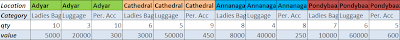
The DatabaseRange is the entire list of information you need to examine, including the field names at the top of the columns.
The FieldName is the name or cell, of the values to pick the Max from, such as "Value Of Stock" or I3.
The CriteriaRange is made up of two types of information.
The first set of information is the name, or names, of the Fields(s) to be used as the basis for selecting the records, such as the category Brand or Wattage.
The second set of information is the actual record, or records, which are to be selected, such as Horizon as a brand name, or 100 as the wattage.
Formatting
No special formatting is needed.
Examples
The largest Value Of Stock of a particular Product of a particular Brand.


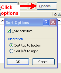
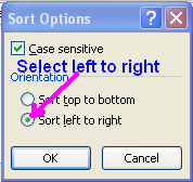


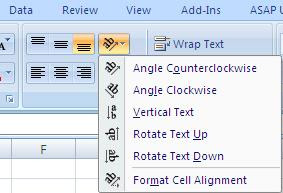
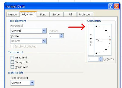
 That’s the Orientation menu. Click on the little drop down arrow beside it.